Efficient grid search via racing with ANOVA models

tune_race_anova() computes a set of performance metrics (e.g. accuracy or RMSE) for a pre-defined set of tuning parameters that correspond to a model or recipe across one or more resamples of the data. After an initial number of resamples have been evaluated, the process eliminates tuning parameter combinations that are unlikely to be the best results using a repeated measure ANOVA model.

Usage

tune_race_anova(object, ...)

# S3 method for class 'model_spec'
tune_race_anova(
  object,
  preprocessor,
  resamples,
  ...,
  param_info = NULL,
  grid = 10,
  metrics = NULL,
  eval_time = NULL,
  control = control_race()
)

# S3 method for class 'workflow'
tune_race_anova(
  object,
  resamples,
  ...,
  param_info = NULL,
  grid = 10,
  metrics = NULL,
  eval_time = NULL,
  control = control_race()
)

Arguments

object: A parsnip model specification or a workflows::workflow().
...: Not currently used.
preprocessor: A traditional model formula or a recipe created using recipes::recipe(). This is only required when object is not a workflow.
resamples: An rset() object that has multiple resamples (i.e., is not a validation set).
param_info: A dials::parameters() object or NULL. If none is given, a parameters set is derived from other arguments. Passing this argument can be useful when parameter ranges need to be customized.
grid: A data frame of tuning combinations or a positive integer. The data frame should have columns for each parameter being tuned and rows for tuning parameter candidates. An integer denotes the number of candidate parameter sets to be created automatically.
metrics: A yardstick::metric_set() or NULL.
eval_time: A numeric vector of time points where dynamic event time metrics should be computed (e.g. the time-dependent ROC curve, etc). The values must be non-negative and should probably be no greater than the largest event time in the training set (See Details below).
control: An object used to modify the tuning process. See control_race() for more details.

Value

An object with primary class tune_race in the same standard format as objects produced by tune::tune_grid().

Details

The technical details of this method are described in Kuhn (2014).

Racing methods are efficient approaches to grid search. Initially, the function evaluates all tuning parameters on a small initial set of resamples. The burn_in argument of control_race() sets the number of initial resamples.

The performance statistics from these resamples are analyzed to determine which tuning parameters are not statistically different from the current best setting. If a parameter is statistically different, it is excluded from further resampling.

The next resample is used with the remaining parameter combinations and the statistical analysis is updated. More candidate parameters may be excluded with each new resample that is processed.

This function determines statistical significance using a repeated measures ANOVA model where the performance statistic (e.g., RMSE, accuracy, etc.) is the outcome data and the random effect is due to resamples. The control_race() function contains are parameter for the significance cutoff applied to the ANOVA results as well as other relevant arguments.

There is benefit to using racing methods in conjunction with parallel processing. The following section shows a benchmark of results for one dataset and model.

Censored regression models

With dynamic performance metrics (e.g. Brier or ROC curves), performance is calculated for every value of eval_time but the first evaluation time given by the user (e.g., eval_time[1]) is analyzed during racing.

Also, values of eval_time should be less than the largest observed event time in the training data. For many non-parametric models, the results beyond the largest time corresponding to an event are constant (or NA).

Benchmarking results

To demonstrate, we use a SVM model with the kernlab package.

library(kernlab)
library(tidymodels)
library(finetune)
library(doParallel)

## -----------------------------------------------------------------------------

data(cells, package = "modeldata")
cells <- cells |> select(-case)

## -----------------------------------------------------------------------------

set.seed(6376)
rs <- bootstraps(cells, times = 25)

We’ll only tune the model parameters (i.e., not recipe tuning):

## -----------------------------------------------------------------------------

svm_spec <-
  svm_rbf(cost = tune(), rbf_sigma = tune()) |>
  set_engine("kernlab") |>
  set_mode("classification")

svm_rec <-
  recipe(class ~ ., data = cells) |>
  step_YeoJohnson(all_predictors()) |>
  step_normalize(all_predictors())

svm_wflow <-
  workflow() |>
  add_model(svm_spec) |>
  add_recipe(svm_rec)

set.seed(1)
svm_grid <-
  svm_spec |>
  parameters() |>
  grid_latin_hypercube(size = 25)

We’ll get the times for grid search and ANOVA racing with and without parallel processing:

## -----------------------------------------------------------------------------
## Regular grid search

system.time({
  set.seed(2)
  svm_wflow |> tune_grid(resamples = rs, grid = svm_grid)
})

##    user  system elapsed
## 741.660  19.654 761.357

## -----------------------------------------------------------------------------
## With racing

system.time({
  set.seed(2)
  svm_wflow |> tune_race_anova(resamples = rs, grid = svm_grid)
})

##    user  system elapsed
## 133.143   3.675 136.822

Speed-up of 5.56-fold for racing.

## -----------------------------------------------------------------------------
## Parallel processing setup

cores <- parallel::detectCores(logical = FALSE)
cores

## [1] 10

cl <- makePSOCKcluster(cores)
registerDoParallel(cl)

## -----------------------------------------------------------------------------
## Parallel grid search

system.time({
  set.seed(2)
  svm_wflow |> tune_grid(resamples = rs, grid = svm_grid)
})

##  user  system elapsed
## 1.112   0.190 126.650

Parallel processing with grid search was 6.01-fold faster than sequential grid search.

## -----------------------------------------------------------------------------
## Parallel racing

system.time({
  set.seed(2)
  svm_wflow |> tune_race_anova(resamples = rs, grid = svm_grid)
})

##  user  system elapsed
## 1.908   0.261  21.442

Parallel processing with racing was 35.51-fold faster than sequential grid search.

There is a compounding effect of racing and parallel processing but its magnitude depends on the type of model, number of resamples, number of tuning parameters, and so on.

References

Kuhn, M 2014. "Futility Analysis in the Cross-Validation of Machine Learning Models." https://arxiv.org/abs/1405.6974.

Examples

# \donttest{
library(parsnip)
library(rsample)
library(dials)
#> Loading required package: scales

## -----------------------------------------------------------------------------

if (rlang::is_installed(c("discrim", "lme4", "modeldata"))) {
  library(discrim)
  data(two_class_dat, package = "modeldata")

  set.seed(6376)
  rs <- bootstraps(two_class_dat, times = 10)

  ## -----------------------------------------------------------------------------

  # optimize an regularized discriminant analysis model
  rda_spec <-
    discrim_regularized(frac_common_cov = tune(), frac_identity = tune()) |>
    set_engine("klaR")

  ## -----------------------------------------------------------------------------

  ctrl <- control_race(verbose_elim = TRUE)
  set.seed(11)
  grid_anova <-
    rda_spec |>
    tune_race_anova(Class ~ ., resamples = rs, grid = 10, control = ctrl)

  # Shows only the fully resampled parameters
  show_best(grid_anova, metric = "roc_auc", n = 2)

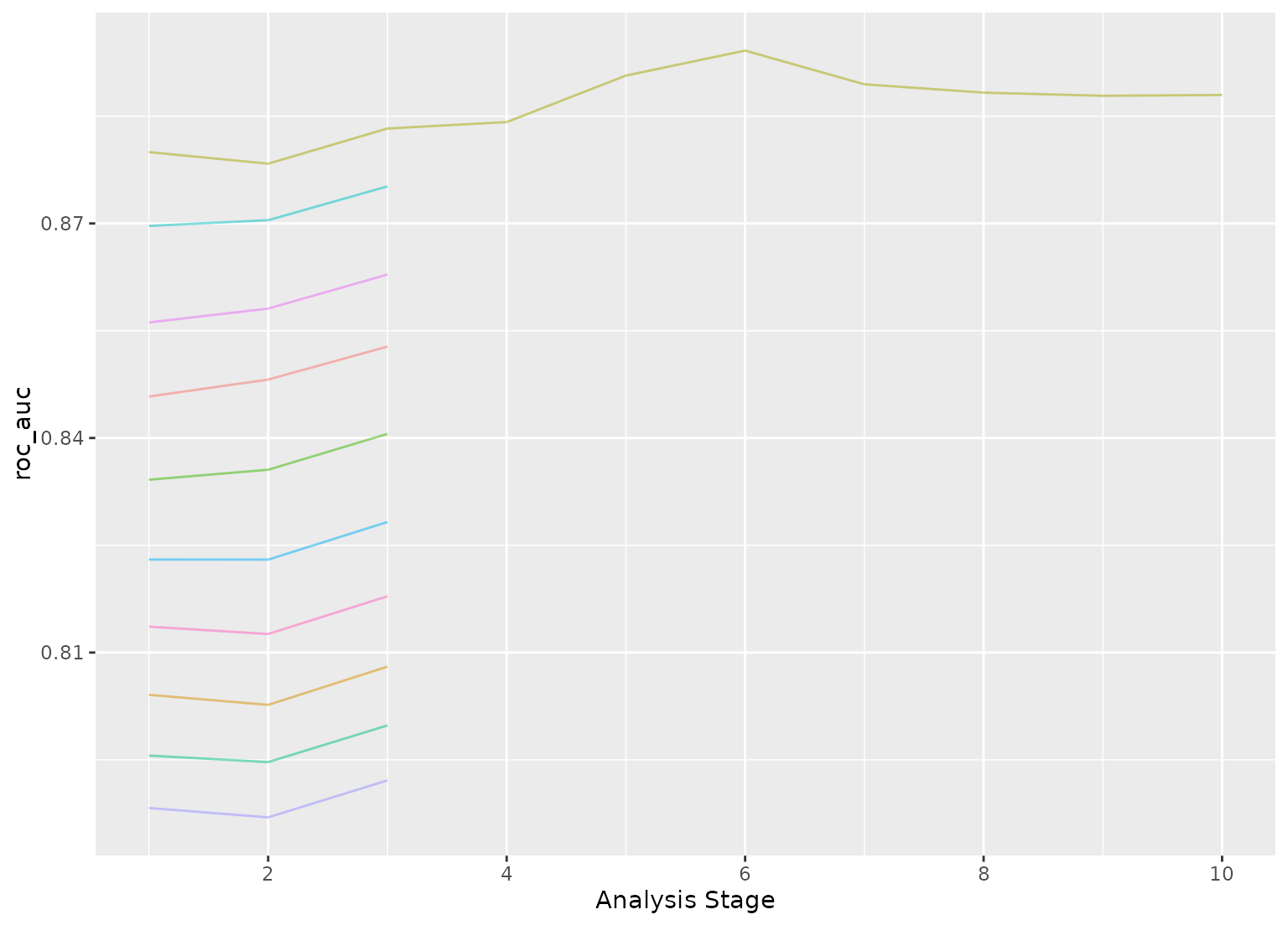
  plot_race(grid_anova)
}
#> 
#> Attaching package: ‘discrim’
#> The following object is masked from ‘package:dials’:
#> 
#>     smoothness
#> ℹ Evaluating against the initial 3 burn-in resamples.
#> ℹ Racing will maximize the roc_auc metric.
#> ℹ Resamples are analyzed in a random order.
#> ℹ Bootstrap05: All but one parameter combination were eliminated.

# }